

![]()
A fast Python library for multi-dimensional Chebyshev tensor interpolation with analytical derivatives
PyChebyshev provides a fully optimized Python implementation of the Chebyshev tensor method, demonstrating that it achieves comparable speed and accuracy to the state-of-the-art MoCaX C++ library for European option pricing via Black-Scholes — with pure Python and NumPy only.
Based on standardized 5D Black-Scholes tests (test_5d_black_scholes() with S, K, T, σ, r):
| Method | Price Error | Greek Error | Build Time | Query Time | Notes |
|---|---|---|---|---|---|
| Analytical | 0.000% | 0.000% | N/A | ~10μs | Ground truth (blackscholes library) |
| Chebyshev Barycentric | 0.000% | 1.980% | ~0.35s | ~0.065ms | Full tensor, analytical derivatives |
| Chebyshev TT | 0.014% | 0.029% | ~0.35s | ~0.004ms | TT-Cross, ~7,400 evals (vs 161k full) |
| MoCaX Standard | 0.000% | 1.980% | ~1.04s | ~0.47ms | Proprietary C++, full tensor (161k evals) |
| MoCaX TT | 0.712% | 1.604% | ~5.73s | ~0.25ms | Proprietary C++, ALS (8k evals) |
| FDM | 0.803% | 2.234% | N/A | ~0.5s/case | PDE solver, no pre-computation |
Key Insights:
- Chebyshev Barycentric: spectral accuracy (0.000% price error) with analytical derivatives
- Chebyshev TT: only 7,400 evaluations (vs 161,051 full tensor), 50x more accurate than MoCaX TT
- Build time: 0.35s (PyChebyshev) vs 1.04--5.73s (MoCaX)
- Query time: 0.004ms batch (TT) / 0.065ms single (barycentric) vs 0.25--0.47ms (MoCaX)
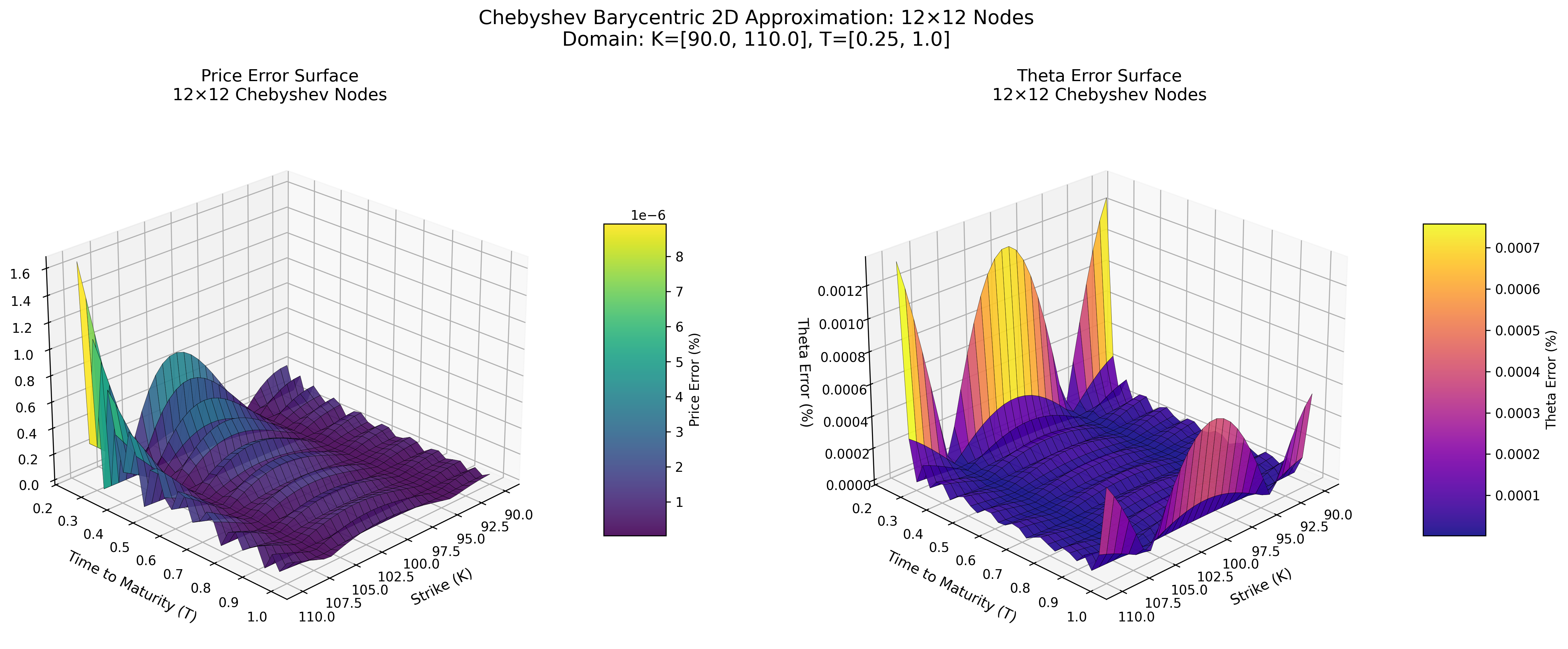
Chebyshev Barycentric (Python)
MoCaX Standard (C++)
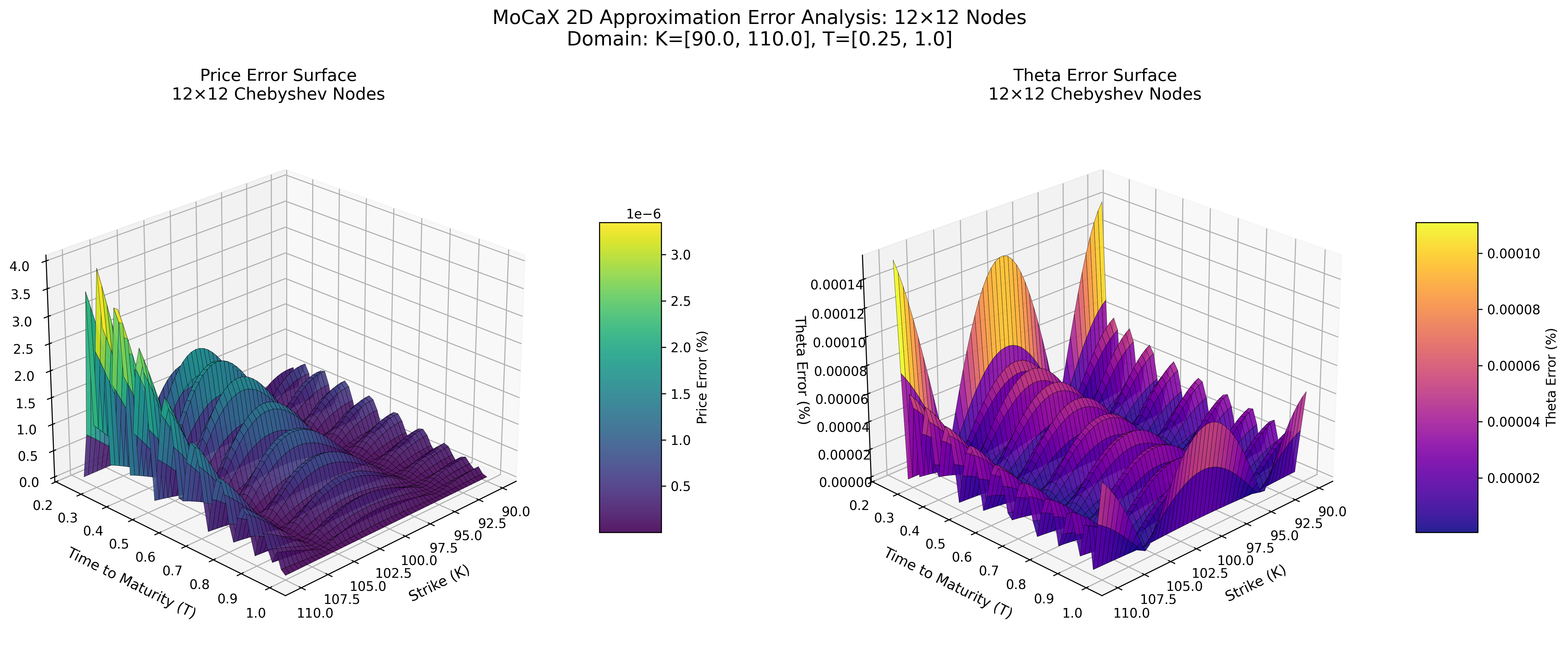
Both methods achieve spectral accuracy (exponential error decay) with identical node configurations, demonstrating that the pure Python implementation successfully replicates the MoCaX algorithm's mathematical foundation.
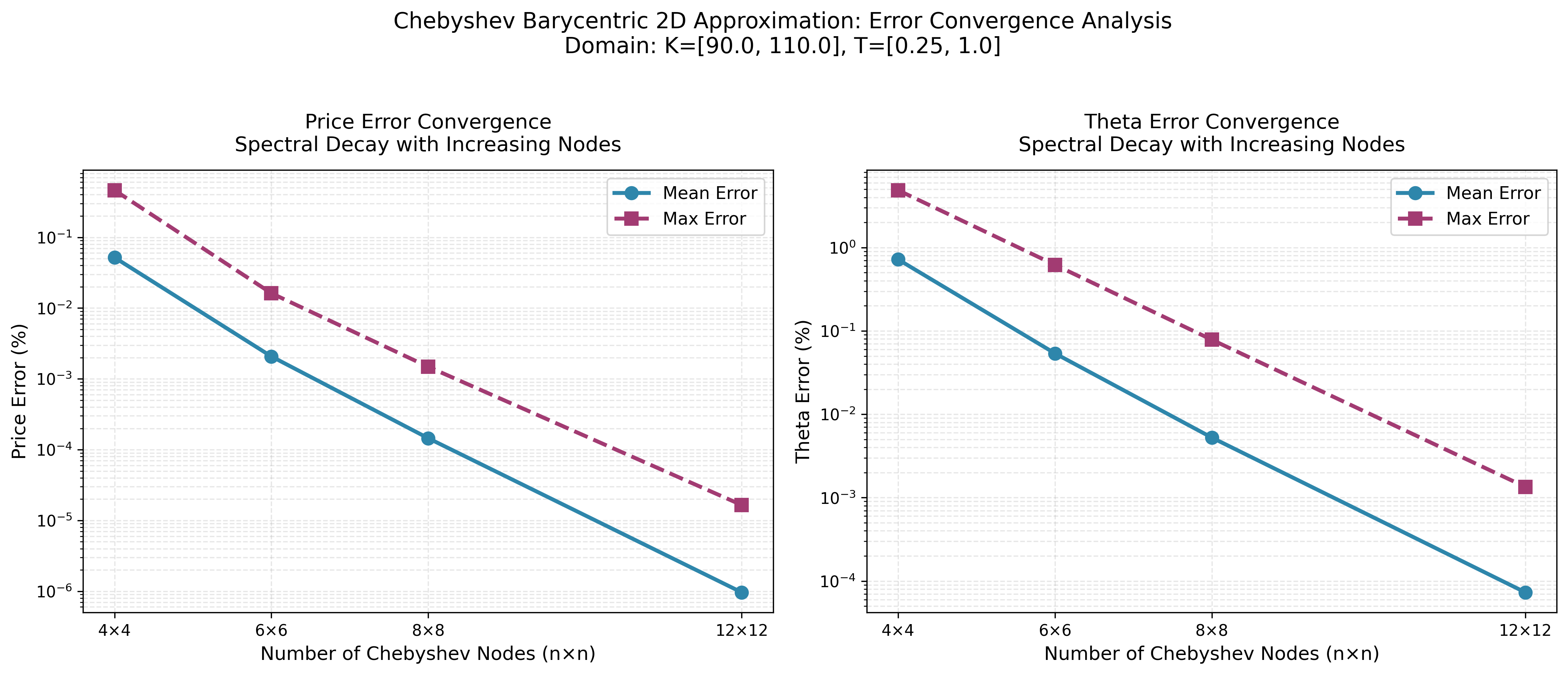
Chebyshev Barycentric
MoCaX Standard
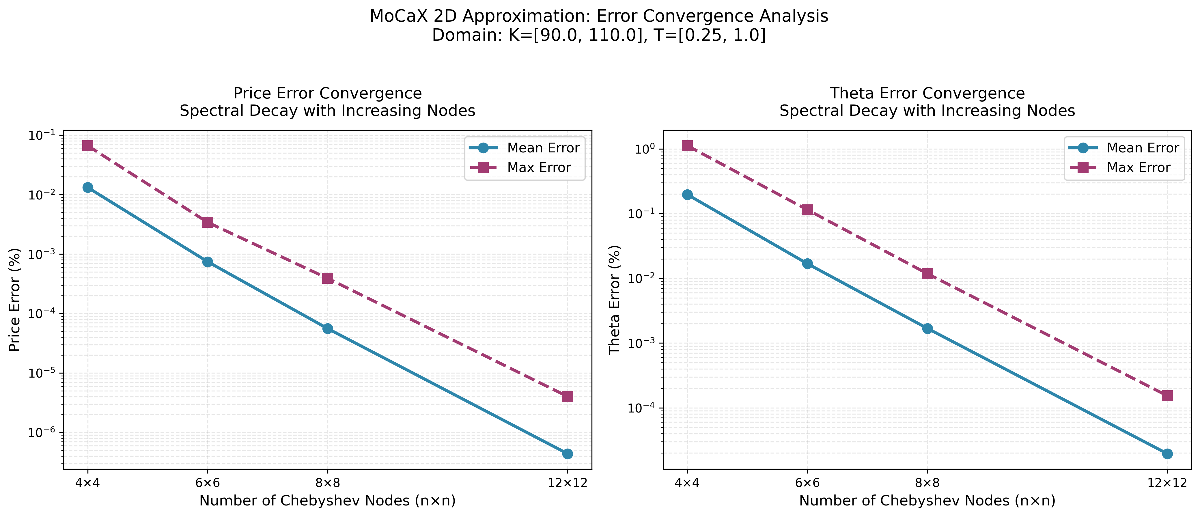
The convergence plots demonstrate exponential error decay as node count increases, confirming the spectral accuracy predicted by the Bernstein Ellipse Theorem. Errors drop rapidly from 4×4 to 12×12 nodes, reaching near-machine precision for this analytic function.
- Full tensor interpolation via
ChebyshevApproximation— spectral accuracy for up to ~5 dimensions - Piecewise Chebyshev (splines) via
ChebyshevSpline— knots at kinks/discontinuities restore spectral convergence for non-smooth functions - Tensor Train decomposition via
ChebyshevTT— TT-Cross builds from O(d·n·r²) evaluations for 5+ dimensions - Sliding technique via
ChebyshevSlider— additive decomposition for separable high-dimensional functions - Arithmetic operators (
+,-,*,/) — combine interpolants into portfolio-level proxies with no re-evaluation - Extrusion & slicing — add or fix dimensions to combine interpolants across different risk-factor sets
- Integration, rootfinding & optimization — spectral calculus directly on interpolants, no re-evaluation needed
- Analytical derivatives via spectral differentiation matrices (no finite differences)
- Vectorized evaluation using BLAS matrix-vector products (~0.065ms/query)
- Pure Python — NumPy + SciPy only, no compiled extensions needed
Special thanks to MoCaX for their high-quality videos on YouTube explaining the mathematical foundations behind their library. These resources were invaluable for understanding and implementing the barycentric Chebyshev interpolation algorithm.
pip install pychebyshevimport math
from pychebyshev import ChebyshevApproximation
# Approximate any smooth function
def my_func(x, _):
return math.sin(x[0]) * math.exp(-x[1])
cheb = ChebyshevApproximation(
my_func,
num_dimensions=2,
domain=[[-1, 1], [0, 2]],
n_nodes=[15, 15],
)
cheb.build()
# Evaluate function value
value = cheb.vectorized_eval([0.5, 1.0], [0, 0])
# Analytical first derivative w.r.t. x[0]
dfdx = cheb.vectorized_eval([0.5, 1.0], [1, 0])
# Price + all derivatives at once (shared weights, ~25% faster)
results = cheb.vectorized_eval_multi(
[0.5, 1.0],
[[0, 0], [1, 0], [0, 1], [2, 0]],
)For 5+ dimensional functions where full tensor grids are too expensive, use ChebyshevTT with TT-Cross:
from pychebyshev import ChebyshevTT

tt = ChebyshevTT(
    my_func, num_dimensions=5,
    domain=[[-1, 1]] * 5,
    n_nodes=[11] * 5,
    max_rank=10,
)
tt.build()
val = tt.eval([0.5] * 5)

# Batch evaluation (much faster per point)
import numpy as np
points = np.random.uniform(-1, 1, (1000, 5))
vals = tt.eval_batch(points)
Note:
ChebyshevTTuses finite differences for derivatives (not analytical spectral differentiation). First-order Greeks are typically accurate to ~0.03%; see the docs for details.
For functions that decompose additively, use ChebyshevSlider:
from pychebyshev import ChebyshevSlider

slider = ChebyshevSlider(
    my_func, num_dimensions=10,
    domain=[[-1, 1]] * 10,
    n_nodes=[11] * 10,
    partition=[[0, 1], [2, 3], [4, 5], [6, 7], [8, 9]],
    pivot_point=[0.0] * 10,
)
slider.build()
val = slider.eval([0.5] * 10, [0] * 10)
See the documentation for full API reference and usage guides.
PyChebyshev uses Chebyshev tensor interpolation to pre-compute fast approximations of smooth functions. The approach generalizes to all analytic functions, as proven by Gaß et al. (2018), which establishes (sub)exponential convergence rates for Chebyshev interpolation of parametric conditional expectations.
| Class | Approach | Build Cost | Eval Cost | Derivatives |
|---|---|---|---|---|
ChebyshevApproximation |
Full tensor + barycentric weights |
|
|
Analytical (spectral) |
ChebyshevSpline |
Piecewise Chebyshev at knots |
|
|
Analytical (per piece) |
ChebyshevTT |
TT-Cross + maxvol pivoting |
|
|
Finite differences |
ChebyshevSlider |
Additive decomposition into slides | Sum of slide grids | Sum of per-slide evals | Analytical (per-slide) |
Barycentric interpolation (ChebyshevApproximation): The barycentric formula separates node positions from function values — weights
Tensor Train decomposition (ChebyshevTT): The full
BLAS vectorization: All evaluation paths route tensor contractions through optimized BLAS routines (numpy.dot, numpy.einsum), achieving ~150x speedup over scalar loops.
For the full mathematical foundation — Chebyshev nodes, Bernstein ellipse theorem, barycentric formula, spectral differentiation matrices, and TT-Cross algorithm — see the documentation.