Single-cell causal network inference based on neighbor cross-mapping entropy
2024/04/24 Update!!!
The Python version significantly improved the computation speed.
If you are familar with Shell and Python, and want to run this algorithm on the server, please check the pyNME folder https://github.com/LinLi-0909/NME/tree/main/pyNME .
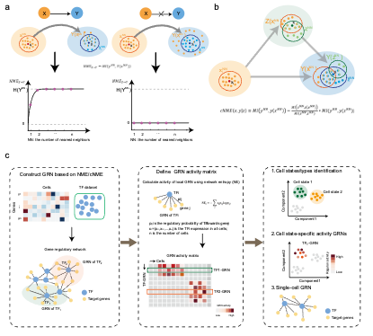
Gene regulatory networks (GRNs) reveal the complex molecular interactions that govern cell state. However, it is challenging for identifying causal
relations among genes due to noisy data and molecular nonlinearity. Here, we propose a novel causal criterion, neighbor cross-mapping entropy (NME)
for inferring GRNs from both steady data and time-series data. NME is designed to quantify “continuous causality” or
functional dependency from one variable to another based on their function continuity with varying neighbor sizes.
NME shows superior performance on benchmark datasets, comparing with existing methods.
By applying to scRNA-seq datasets, NME not only reliably inferred GRNs for cell types but also identified cell states.
Based on the inferred GRNs and further their activity matrices, NME showed better performance in single-cell clustering and downstream analyses.
In summary, based on continuous causality, NME provides a powerful tool in inferring causal regulations of GRNs between genes from scRNA-seq data,
which is further exploited to identify novel cell types/states and predict cell type-specific network modules.
NME is designed based on matlab.
%linux
cd /path/to/NME/Code
filename=../Data/NME_input_data.csv
# the number of mapping neighbors
p=15
# the number of estimating neighbors
k=5
matlab -nodesktop -nosplash -r "filename='$filename',p=$p,k=$k;calc_NME;quit"% matlab
input_data = importdata(filename);
x = input_data(:,1);
y = input_data(:,2);
p=15;
k=5;
out_x2y = DMI(x,y,p,k);
out_y2x = DMI(y,x,p,k);
disp(['The normalized causality from V1 to V2 is:',num2str(out_x2y)]);
disp(['The normalized causality from V2 to V1 is:',num2str(out_y2x)]);filename=../Data/cNME_input_data.tsv
# save cNME output to
output='../Output/example_cNME_output'
# the nubmer of conditional variables
nz=1
# the number of mapping neighbors
p=5
# the number of estimating neighbors
k=5
matlab -nodesktop -nosplash -r "filename='$filename',nz=$nz,p=$p,k=$k,output='$output';calc_cNME;quit"%matlab
filename=../Data/cNME_input_data.tsv
output='../Output/example_cNME_output'
# the nubmer of conditional variables
nz=1
# the number of mapping neighbors
p=5
# the number of estimating neighbors
k=5
input_data = importdata(filename);
var_names = strip(input_data.textdata,'"');
input_data = input_data.data;
out_mat = Get_cDMI(input_data,var_names,var_names,nz,p,k);
out = array2table(out_mat,'VariableNames',var_names,'RowNames',var_names);
writetable(out,[output,'.csv'],'WriteRowNames',true);filename=../Data/scNME_input_data.csv
# save cNME output to
output='../Output/example_scNME_output'
# the number of mapping neighbors
p=15
# species ='human' or 'mouse'
species='human'
# ncpu for paralell calculating
nworkers=20
# set the pcutoff of Hypothesis testing
p_cutoff=0.05
# save scNME output to
output='../Output/example_scNME_output'
matlab -nodesktop -nosplash -r "filename='$filename',species='$species',nz=$nz,p=$p,k=$k,p_cutoff=$p_cutoff,output='$output',nworkers=$nworkers;calc_scNME;quit"scRNA-seq from Seurat objects,e.g.pbmc3k which can be download from https://cf.10xgenomics.com/samples/cell/pbmc3k/pbmc3k_filtered_gene_bc_matrices.tar.gz
%linux
tar zxvf pbmc3k_filtered_gene_bc_matrices.tar.gz
cd filtered_gene_bc_matrices/
%R
library(dplyr)
library(Seurat)
library(patchwork)
# Load the PBMC dataset
pbmc.data <- Read10X(data.dir = "hg19/")
# Initialize the Seurat object with the raw (non-normalized data).
pbmc <- CreateSeuratObject(counts = pbmc.data, project = "pbmc3k", min.cells = 3, min.features = 200)
pbmc
# The [[ operator can add columns to object metadata. This is a great place to stash QC stats
pbmc[["percent.mt"]] <- PercentageFeatureSet(pbmc, pattern = "^MT-")
pbmc <- NormalizeData(pbmc, normalization.method = "LogNormalize", scale.factor = 10000)
##Selected variable genes to construct scNME
pbmc <- FindVariableFeatures(pbmc, selection.method = "vst", nfeatures = 5000)
variable_genes <- VariableFeatures(pbmc)
tf <- read.csv('human_tf_trrust.txt',header=F)##can be download from https://github.com/LinLi-0909/NME/tree/main/data
genes <- unique(c(variable_genes,tf$V1))
data <- GetAssayData(pbmc,slot = 'data')
data_f <- data[rownames(data)%in%genes,]
write.csv(data_f,'data_f.csv')
%matlab
GEM = importdata('data_f.csv');
cellnames = GEM.textdata(1,2:end);
gene_names = GEM.textdata(2:end,1);
regulators = importdata('human_tf_trrust.txt');
[~,pos] = ismember(regulators,gene_names);
pos(pos==0)=[];
GEM = GEM.data;
GEM = GEM';
nz=1;
p=12;
l=5;
Net = Get_cDMI(GEM,regulators,gene_names,nz,p,l);%% causal network
%% compute the tf-GRN activity of cells(entropy),and binary causal network (bnet)
p_value=0.1 % 0.05,0.01
[entropy,bnet,regulators] = Get_entropy(GEM,Net,regulators,gene_names,p_value)
scNME_matrix  = array2table(entropy','RowNames',gene_names(pos),'VariableNames',cellnames);
writetable(scNME_matrix,'scNME_matrix.csv','WriteRowNames',true);
net_sig = array2table(bnet,'RowNames',gene_names(pos),'VariableNames',gene_names);
writetable(net_sig,'binary_net.csv','WriteRowNames',true);
%matalab (for large datasets)
here, we calculate the causal network of genes, respectively. For example, there are 6,000 genes in GEM.
We can divide the genes into 10 sets(or 5, 12 sets which can be defined yourself) , e.g. 1:600, 601:1200,...,5401:6000.
And for each gene set, we can calculate the causal network.
%e.g. for 1:600 genes
GEM = importdata('data_f.csv');
cellnames = GEM.textdata(1,2:end);
gene_names = GEM.textdata(2:end,1);
regulators = importdata('human_tf_trrust.txt');
[~,pos] = ismember(regulators,gene_names);
pos(pos==0)=[];
GEM = GEM.data;
GEM = GEM';
nz=1;
p=12;
l=5;
timeseries=0;
ns=1;%the gene index
ne=600;%the gene idex
net1 = Get_cDMI_par(GEM,regulators,gene_names,nz,p,l,timeseries,ns,ne)%% causal network for tfs and 1:600 genes
save('net1.mat','net1')
%e.g. for 601:1200 genes
GEM = importdata('data_f.csv');
cellnames = GEM.textdata(1,2:end);
gene_names = GEM.textdata(2:end,1);
regulators = importdata('human_tf_trrust.txt');
[~,pos] = ismember(regulators,gene_names);
pos(pos==0)=[];
GEM = GEM.data;
GEM = GEM';
nz=1;
p=12;
l=5;
timeseries=0;
ns=601;%the gene index
ne=1200;%the gene idex
net2 = Get_cDMI_par(GEM,regulators,gene_names,nz,p,l,timeseries,ns,ne)%% causal network for tfs and 601:1200 genes
save('net2.mat','net2')
......
%for 5401:6000
GEM = importdata('data_f.csv');
cellnames = GEM.textdata(1,2:end);
gene_names = GEM.textdata(2:end,1);
regulators = importdata('human_tf_trrust.txt');
[~,pos] = ismember(regulators,gene_names);
pos(pos==0)=[];
GEM = GEM.data;
GEM = GEM';
nz=1;
p=12;
l=5;
timeseries=0;
ns=5401;%the gene index
ne=6000;%the gene idex
net10 = Get_cDMI_par(GEM,regulators,gene_names,nz,p,l,timeseries,ns,ne)%% causal network for tfs and 5401:6000 genes
save('net10.mat','net10')
load('net1.mat');load('net2.mat');load('net3.mat');load('net4.mat');load('net5.mat');
load('net6.mat');load('net7.mat');load('net8.mat');load('net9.mat');load('net10.mat');
Net=[net1,net2,net3,net4,net5,net6,net7,net8,net9,net10];
%% compute the tf-GRN activity of cells(entropy),and binary causal network (bnet)
p_value=0.1 % 0.05,0.01
[entropy,bnet,regulators] = Get_entropy(GEM,Net,regulators,gene_names,p_value)
scNME_matrix  = array2table(entropy','RowNames',gene_names(pos),'VariableNames',cellnames);
writetable(scNME_matrix,'scNME_matrix.csv','WriteRowNames',true);
net_sig = array2table(bnet,'RowNames',gene_names(pos),'VariableNames',gene_names);
writetable(net_sig,'binary_net.csv','WriteRowNames',true);
%R
entropy_count <- read.csv('scNME_matrix.csv',header=T,row.names=1)
colnames(entropy_count)<- colnames(pbmc)
gene = rownames(entropy_count)
x = apply(entropy_count,1,function(x){sum(x!=0)})
gene = paste(gene,'(',x,'g)',sep = '')
rownames(entropy_count)<- gene
entropy_S <- CreateSeuratObject(counts =entropy_count,min.cells = 3,min.features = 1)
entropy_S
entropy_S@assays$RNA@data<- entropy_S@assays$RNA@counts
entropy_S$cluster <- pbmc$seurat_clusters
Idents(entropy_S)<- entropy_S$cluster
diff_GRN <- FindAllMarkers(entropy_S,logfc.threshold = 0.25,only.pos = T)
diff_GRN %>%
  group_by(cluster) %>%
  slice_head(n = 10) %>%
  ungroup() -> top10
DotPlot(entropy_S, features = top10$gene,group.by = 'cluster',dot.scale = 10,dot.min=0)+RotatedAxis()+
  scale_x_discrete("")+scale_y_discrete()+scale_color_gradientn(colours = rev(c("chocolate","white","slateblue")))+
  scale_size_continuous(range=c(5, 11))+theme(panel.grid = element_line(color="lightgrey"))