This package estimates linear models with high dimensional categorical variables and/or instrumental variables.

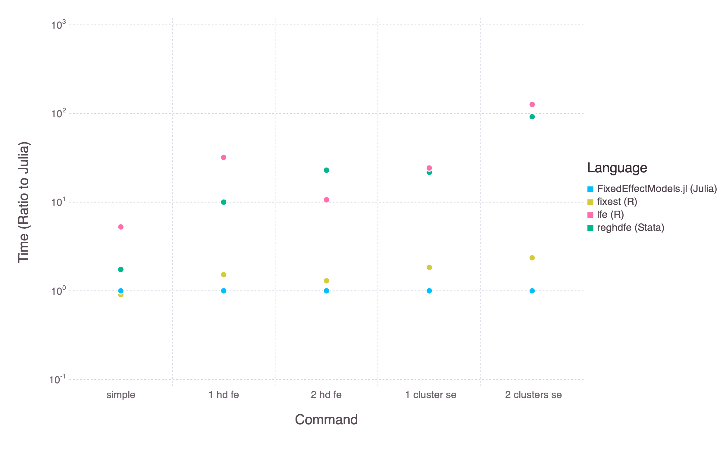
Its objective is similar to the Stata command reghdfe and the R function felm. The package is usually much faster than these two options.

Estimate a model

To estimate a @model, specify a formula with, eventually, a set of fixed effects with the argument fe, a way to compute standard errors with the argument vcov, and a weight variable with weights.

using DataFrames, RDatasets, FixedEffectModels
df = dataset("plm", "Cigar")
df[:StateCategorical] =  categorical(df[:State])
df[:YearCategorical] =  categorical(df[:Year])
reg(df, @model(Sales ~ NDI, fe = StateCategorical + YearCategorical, weights = Pop, vcov = cluster(StateCategorical)))
# =====================================================================
# Number of obs:               1380   Degrees of freedom:            31
# R2:                         0.804   R2 within:                  0.139
# F-Statistic:              13.3481   p-value:                    0.000
# Iterations:                     6   Converged:                   true
# =====================================================================
#         Estimate  Std.Error  t value Pr(>|t|)   Lower 95%   Upper 95%
# ---------------------------------------------------------------------
# NDI  -0.00526264 0.00144043 -3.65351    0.000 -0.00808837 -0.00243691
# =====================================================================

• A typical formula is composed of one dependent variable, exogeneous variables, endogeneous variables, and instrumental variables.

   dependent variable ~ exogenous variables + (endogenous variables ~ instrumental variables)

• Fixed effect variables are indicated with the keyword argument fe. They must be of type CategoricalArray (use categorical to convert a variable to a CategoricalArray).

   df[:StateCategorical] =  categorical(df[:State])
   # one high dimensional fixed effect
   fe = StateCategorical

  You can add an arbitrary number of high dimensional fixed effects, separated with +

   df[:YearCategorical] =  categorical(df[:Year])
   fe = StateCategorical + YearCategorical

  Interact multiple categorical variables using &

   fe = StateCategorical&DecPooled

  Interact a categorical variable with a continuous variable using &

   fe = StateCategorical + StateCategorical&Year

  Alternative, use * to add a categorical variable and its interaction with a continuous variable

   fe = StateCategorical*Year
   # equivalent to fe = StateCategorical + StateCategorical&year

• Standard errors are indicated with the keyword argument vcov.

   vcov = robust
   vcov = cluster(StateCategorical)
   vcov = cluster(StateCategorical + YearCategorical)

• weights are indicated with the keyword argument weights

   weights = Pop

Arguments of @model are captured and transformed into expressions. If you want to program with @model, use expression interpolations:

using DataFrames, RDatasets, FixedEffectModels
df = dataset("plm", "Cigar")
w = :Pop
reg(df, @model(Sales ~ NDI, weights = $(w)))

Output

reg returns a light object. It is composed of

• the vector of coefficients & the covariance matrix
• a boolean vector reporting rows used in the estimation
• a set of scalars (number of observations, the degree of freedoms, r2, etc)
• with the option save = true, a dataframe aligned with the initial dataframe with residuals and, if the model contains high dimensional fixed effects, fixed effects estimates.

Methods such as predict, residuals are still defined but require to specify a dataframe as a second argument. The problematic size of lm and glm models in R or Julia is discussed here, here, here here (and for absurd consequences, here and there).

You may use RegressionTables.jl to get publication-quality regression tables.

Solution Method

Denote the model y = X β + D θ + e where X is a matrix with few columns and D is the design matrix from categorical variables. Estimates for β, along with their standard errors, are obtained in two steps:

1. y, X are regressed on D using the package FixedEffects.jl
2. Estimates for β, along with their standard errors, are obtained by regressing the projected y on the projected X (an application of the Frisch Waugh-Lovell Theorem)
3. With the option save = true, estimates for the high dimensional fixed effects are obtained after regressing the residuals of the full model minus the residuals of the partialed out models on D using the package FixedEffects.jl

Parallel / multi-threading

The package has support for parallel computing and multi-threading. In this case, each regressor is demeaned in a different processor/thread. It only allows for a modest speedup (between 10% and 60%) since the demeaning operation is typically memory bound.

1. For parallel computing, the syntax is as follow:

   using Distributed
   addprocs(n)
   @everywhere using DataFrames, FixedEffectModels
   reg(df, @model(Sales ~ NDI, fe = StateCategorical + YearCategorical), method = :lsmr_parallel)

2. For multi-threading, before starting Julia, set the number of threads to n with

   export JULIA_NUM_THREADS=n
   

   Then, in Julia, use the option lsmr_threads

   using DataFrames, FixedEffectModels
   reg(df, @model(Sales ~ NDI, fe = StateCategorical + YearCategorical), method = :lsmr_threads)

References

Baum, C. and Schaffer, M. (2013) AVAR: Stata module to perform asymptotic covariance estimation for iid and non-iid data robust to heteroskedasticity, autocorrelation, 1- and 2-way clustering, and common cross-panel autocorrelated disturbances. Statistical Software Components, Boston College Department of Economics.

Correia, S. (2014) REGHDFE: Stata module to perform linear or instrumental-variable regression absorbing any number of high-dimensional fixed effects. Statistical Software Components, Boston College Department of Economics.

Fong, DC. and Saunders, M. (2011) LSMR: An Iterative Algorithm for Sparse Least-Squares Problems. SIAM Journal on Scientific Computing

Gaure, S. (2013) OLS with Multiple High Dimensional Category Variables. Computational Statistics and Data Analysis

Kleibergen, F, and Paap, R. (2006) Generalized reduced rank tests using the singular value decomposition. Journal of econometrics

Kleibergen, F. and Schaffer, M. (2007) RANKTEST: Stata module to test the rank of a matrix using the Kleibergen-Paap rk statistic. Statistical Software Components, Boston College Department of Economics.